Predecessor search for Big Data: x-fast tries, locality of reference and all that

Abstract: An intro to data structures with locality of reference-type features. We review x-fast tries in some detail and then talk about similar data structures, where they shine and where they don’t

Consider a set {n} of n integers within the range 0..u-1. Let’s assume we need to build a data structure that allows for performing of the following operations efficiently:

Look up: check if an integer x is in {n}
Update: Insert an integer into {n} or delete one.

Let’s check out how some common data structures are holding up with these: a simple sorted array, a balanced binary search tree (whether it is AVL or red-black), and a hash table:

	Lookup	Update
Sorted Array	Ө(log(n))	O(n)
Balanced binary tree	Ө(log(n))	Ө(log(n))
Hash Table	Ө(1)	Ө(1)

The hash table is designed to be optimal for these two operations so it is the best fit here. But what if we modify the search operation a little bit and require returning of the next closest element if the exact value is not within the set {n}? So that for 69 in {1,55,68, 100} we would want to get 68 as it is close enough. One can see how the need for such a modification can arise in applications.

We can think of a couple of similar problem modifications: return the closest element, or only the next closest element that is greater than the query value (they call this the successor element search in the literature), or the closest one that is smaller (predecessor search). One can see that these problems overlap and can be reformulated in terms of each other, so let’s just start with implementing one of them:

Find predecessor item: look up an integer x and if it is not in the set, return the closest int within the set that is lower by value

Here is how we can implement Predecessor Search for the data structures we considered above:

Sorted Array we search for the value using binary search and if turns out that it is not within the set, we simply take the next left value from where it should have been.
Search Tree approach is similar to Sorted Array: we traverse to the next item left from where the value should have been
Hash Table: if the value x is not within the set, the only option is to look up x-1 and continue looking up lower values until we stumble upon one within the set. The average distance between the two values is asymptotically Ө(u/n).

	Lookup	Update	Predeccessor
Sorted Array	Ө(log(n))	O(n)	O(log(n))
Balanced binary tree	Ө(log(n))	Ө(log(n))	O(log(n))
Hash Table	Ө(1)	Ө(1)	O(u/n)

We see that the advantages of the plain hash table disappear when it comes to predecessor search. Can we think of a way to improve the hash table’s performance here?

One way that may come to mind at this point is to just store pointers to predecessor and successor elements for each of the the elements within u right in the hash table.

This would enable quick predecessor lookup, but would break the performance of the Update function. Adding a value for this Hash-Table with Predecessor Pointers means we need to update the predecessor pointers for all values from the new one to the closest larger one. Which, again, means O(u/n) operations.

There is another drawback to this approach. Now we have to store not just n set elements but all the u possible values. Additionally, pointer size is bound by log(u) needed to store the value position. So the total size of the structure now depends on u as well.

We can sum it up with this:

	Lookup	Update	Predeccessor	Size
Sorted Array	Ө(log(n))	O(n)	O(log(n))	Ө(n)
Balanced binary tree	Ө(log(n))	Ө(log(n))	O(log(n))	Ө(n)
Hash Table	Ө(1)	Ө(1)	Ө(u/n)	Ө(n)
Hash-Table with Predecessor Pointers	Ө(1)	Ө(1)	Ө(u/n)	Ө(u log(u))

Some Reflection

Let’s reflect on these results a little bit. We see that hash table is ideal when we look up exact values but breaks down when we start inquiring on operations where locality of the value starts to matter.

That makes sense. A proper hash function means a mathematically unstable one: even small increments change the hash completely which insures the values are spread homogeneously among the hash table buckets.

At the same time we see that binary search tree-style data structures are quite resielent to locality context class of problem. One can say that search tree is based on the concept of proximity and contains the information about locality.

X-fast trie is a data structure that combines the advantages of both search trees and hash tables.

Enter X-fast trie

Let’s build a bitwise search tree on top of all the u elements. All the u values are at the tree’s leaves (which makes this search tree a trie). Let’s mark all those tree nodes where there is an ancestor leave which is within {n} as “black” and the rest of the nodes keep “white”.

Here is a nice illustrating graph from opendatastructures.org:

x-fast

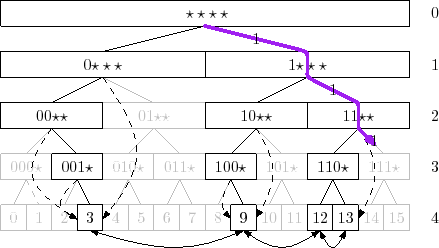
Now we can implement the operations like this:

Predecessor: there is log(u) nodes within the search tree that are parents to the leave corresponding to the value we look up. If a node is marked with black all the nodes above are black too. That means we have a sorted array of log(u) values corresponding to the i element. We use binary search to find the lowest black element and then traverse down the left side along the black nodes to get to the predecessor value. How much will it cost? Binary search among log(u) values would be Ө(log(log(u))), traversing down to predecessor value: Ө(1).
Update: is quite similar to the simple trie update case. For adding a value, ee traverse through all the parent nodes and “repaint” all of them black. For removing an item, we paint with white all the parent nodes for which no other children leaves are black. So Ө(log(u)).

Memory needed to store the “color” (black or white) bits for all the nodes within the search tree grows steeply: we get 2u-1 nodes for a complete binary trie with u leaves. That is where a hash table comes in, we only the “black”-marked nodes within the hash table for each level of the trie. That means n entries on the leave level, less or equal than n/2 on the second lowest and so on for each of the log(u) hash tables. So the space is bound by Ө(n log(u)).

Let’s sum it up by updating the table

	Lookup	Update	Predecessor	Size
Sorted Array	Ө(log(n))	O(n)	O(log(n))	Ө(n)
Balanced binary tree	Ө(log(n))	Ө(log(n))	O(log(n))	Ө(n)
Hash Table	Ө(1)	Ө(1)	Ө(M/n)	Ө(n)
Hash-Table with Predecessor Pointers	Ө(1)	Ө(1)	Ө(u/n)	Ө(u log(u))
X-fast trie	O(1)	O(log(u))	O(log(log(u)))	O(n log(u))

Toy example

The easiest way to grok how these operations are implemented is to implement them yourself. So I did.

Here is our toy case. With movie and tv show titles such as X-files, X-men and American History X, we have a trope of X standing for something misterious (and heavily implied to be hip). How often are movies with such titles released? What was the first X-movie released since, say 1975?

To find out, let us build the X-fast trie index for such X-titled movies by the year of release.

Let’s consider years from 1950 + 64 = 2004 to be our M= 2^6 - 1=63 range. Here is a plot of what all the M leaves and the color of parent nodes for each of the depth levels:

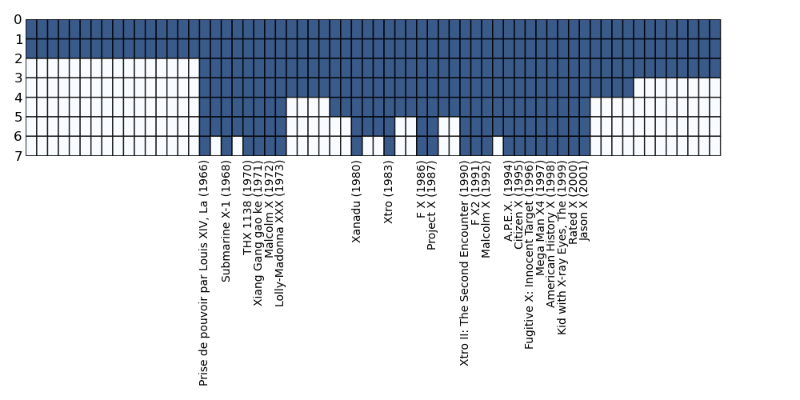
We have total of x levels, where x comes from $u < 2^x -1$. That means we have got x hash functions where we store keys of the “black”-marked nodes. Root level 0 contains only one node, in our case a blue/black one (it is always black as long as there is a single value within {n}). The second lower level, 1, contains two nodes and so on.

In order to look up the predecessor movie for 1975 we start the binary search for the specific level where the nodes turn white by looking up the corresponding node values within the parent nodes. We find out that the level is 3. Then we traverse down along the left side and find the corresponding predecessor movie: Lolly-Maddonna XXXX (1973).

What would it take to add another movie, say, “Not a Real Movie X (1975)”? That would mean we need to go through all the parent nodes and make sure they are added to the corresponding level hash functions.

Practical Examples

Comparing search time asymptotics for X-fast tries and search trees, we see that X-fast shines when log[N] grows faster than log[log[M]], which comes down to the criteria of N >> log[M].

So let’s come up with some practical examples of where X-fast trie can be useful:

Imagine you are developing a flight searching website. For the given datetime of expected departure we return the list of all the upcoming flights. Flights are updated and changed frequently. Datetime minutes can make up all the possible u values, and the flights to a specific direction make up {n} set.
IP/other network protocols Packet Routing: an internet router needs to redirect the IP packets to other routers with the IP closest to the requested one.
Trackless bitTorrent peer-to-peer networks look up content by hash and the nodes with IDs closest to this hash (by some metric) are assigned with tracking that content. X-fast trie can get useful to lookup content in huge networks with large number of nodes (so that n >> log[M]). (Hey! By the way, see my other post on the subject!).

Data Structures with locality of reference

X-fast trie is an example of the data structure where locality of reference is tracked. Another one, more famous one, would of course be the search tree. Together data structures like these compose a large family of cases where some concept of locality matters. The ones used in practice tend to share many features with the x-fast trie case we considered here.

It is easy to see how wide the domain of locality-sensitive applications is. It can be extended to multidimensional cases too. Say, geolocation applications would involve ability to look up objects closest to a specific point. How can one approach this? A search tree can be a good start, but for sufficiently large maps we can devise some equivalent of 2D x-fast trie or move to other fancier solutions.

Pretty nice, huh?